Tutorial - Non-reacting flow past a cylinder
Introduction
PeleLM enables the representation of complex non-Cartesian geometries using an embedded boundary (EB) method. This method relies on intersecting an arbitrary surface with the Cartesian matrix of uniform cells, and modifies the numerical stencils near cells that are cut by the EB.
The goal of this tutorial is to setup a simple 2-dimentional flow past cylinder case in PeleLM. This document provides step by step instructions to properly set-up the domain and boundary conditions, construct an initial solution.
Setting-up your environment
PeleProduction
As explained in section PeleLM Quickstart, PeleLM relies on a number of supporting softwares:
- AMReX is a software frameworks that provides the data structure and enable massive parallelization.
- IAMR is a parallel, adaptive mesh refinement (AMR) code that solves the variable-density incompressible Navier-Stokes equations.
- PelePhysics is a repository of physics databases and implementation code. In particular, the choice of chemistry and transport models as well as associated functions and capabilities are managed in PelePhysics.
All of these codes have their own development cycle, and it can make the setup of a PeleLM run a bit tricky. To simplify the process, PeleProduction will be employed. PeleProduction is a collection of run folders for various Pele codes and processing. It includes git submodules for the dependent codes (such as PeleLM, PelePhysics, AMReX, etc), that can be frozen to a particular commit. This organizational strategy enables to manage the interactions between the various dependent repositories (to keep them all compatible with each other).
Step by step instructions
First, make sure that “git” is installed on your machine—we recommend version 1.7.x or higher. Then, follow these few steps to setup your run environment:
Download the PeleProduction repository and :
git clone https://github.com/AMReX-Combustion/PeleProduction.git

cd PeleProduction
Switch to the TripleFlame branch :
git checkout Tutorials
The first time you do this, you will need to tell git that there are submodules. Git will look at the
.gitmodulesfile in this branch and use that :git submodule init
Finally, get the correct commits of the sub-repos set up for this branch:
git submodule update
You are now ready to build the FlowPastCylinder case associated with this branch. To do so:
cd Tutorials/FlowPastCylinder
And follow the next steps !
Numerical setup
In this section we review the content of the various input files for the flow past cylinder test case. To get additional information about the keywords discussed, the user is referred to section PeleLM control.
Test case and boundary conditions
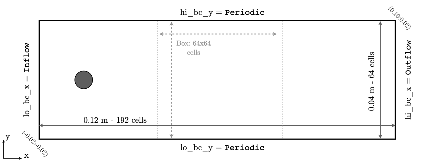
Direct Numerical Simulations (DNS) is performed on a 12x4 \(cm^2\) 2D computational domain, with the bottom left corner located at (-0.02:-0.02) and the top right corner at (0.10:0.02). The base grid is decomposed into 192x64 cells and up to 3 levels of refinement (although we will start with a single level). The refinement ratio between each level is set to 2. The maximum box size is fixed at 64, and the base (level 0) grid is composed of 3 boxes, as shown in Fig 4.
Periodic boundary conditions are used in the transverse (\(y\)) direction, while Inflow (dirichlet) and Outflow (neumann) boundary conditions are used in the main flow direction (\(x\)). The flow goes from left to right.
A cylinder of radius 0.0035 m is placed in the middle of the flow at (0.0:0.0).
 |
The geometry of the problem is specified in the first block of the inputs.2d-regt_VS:
#----------------------DOMAIN DEFINITION------------------------
geometry.is_periodic = 0 0             # Periodicity in each direction: 0 => no, 1 => yes
geometry.coord_sys   = 0               # 0 => cart, 1 => RZ
geometry.prob_lo     = -0.02 -0.02     # x_lo y_lo
geometry.prob_hi     =  0.10  0.02     # x_hi y_hi
The second block determines the boundary conditions. Note that Interior is used to indicate periodic boundary conditions. Refer to Fig 4:
# >>>>>>>>>>>>>  BC FLAGS <<<<<<<<<<<<<<<<
# Interior, Inflow, Outflow, Symmetry,
# SlipWallAdiab, NoSlipWallAdiab, SlipWallIsotherm, NoSlipWallIsotherm
peleLM.lo_bc = Inflow   SlipWallAdiab
peleLM.hi_bc = Outflow  SlipWallAdiab
In the present case, the EB geometry is a simple cylinder (or sphere) which is readily available from the AMReX library and only a few paremeters need to be specified by the user. This is done further down in the input file:
#------------  INPUTS FOR EMBEDED BOUNDARIES ----------------
eb2.geom_type                    = sphere
eb2.sphere_radius                = 0.0035
eb2.sphere_center                = 0.00 0.00
eb2.sphere_has_fluid_inside      = 0
eb2.small_volfrac                = 1.0e-4
Note that the last parameter is used to specify a volume fraction (ratio of the uncovered surface (2D) or volume (3D) over the cell surface or volume) threshold below which a cell is considered fully covered. This prevents the appearance of extremely small partially covered cells which are numerically unstable.
The number of levels, refinement ratio between levels, maximium grid size as well as other related refinement parameters are set under the third block :
#-------------------------AMR CONTROL----------------------------
amr.n_cell          = 192 64     # Level 0 number of cells in each direction
amr.v               = 1          # amr verbosity level
amr.max_level       = 0          # maximum level number allowed
amr.ref_ratio       = 2 2 2 2    # refinement ratio
amr.regrid_int      = 2          # how often to regrid
amr.n_error_buf     = 2 2 2 2    # number of buffer cells in error est
amr.grid_eff        = 0.7        # what constitutes an efficient grid
amr.blocking_factor = 16         # block factor in grid generation
amr.max_grid_size   = 64         # maximum box size
Problem specifications
This very simple problem only has three user-defined problem parameters: the inflow velocity magnitude, the pressure and the temperature. This setup is also constructed to be able to perform the simulation of mixture perturbation crossing over the cylinder so that a switch is available to run this case rather than the simple vortex shedding past a cylinder.
Specifying dirichlet Inflow conditions in PeleLM can seem daunting at first. But it is actually a very flexible process. We walk the user through the details which involve the following files:
pelelm_prob_parm.H, assemble in a C++ structProbParmthe input variables as well as other variables used in the initialization process.pelelm_prob.cpp, initialize and provide default values to the entries ofProbParmand allow the user to pass run-time value using the AMReX parser (ParmParse). In the present case, the parser will read the parameters in thePROBLEM PARAMETERSblock:prob.type = VortexShedding prob.meanFlowMag = 3.0
finally,
pelelm_prob.Hcontains thepelelm_initdataandbcnormalfunctions responsible for generating the initial and boundary conditions, respectively.
Note that in the present case, the default values of pressure and temperature are employed since their respective keywords are not specified in the input file.
Finally, this test uses a constant set of transport parameters rather relying on the EGLib library
(see sec:model:EqSets for more details on EGLib). These transport parameters are specified in the CONSTANT TRANSPORT block:
#------------  INPUTS TO CONSTANT TRANSPORT -----------------
transport.const_viscosity        = 2.0e-04
transport.const_bulk_viscosity   = 0.0
transport.const_conductivity     = 0.0
transport.const_diffusivity      = 0.0
Only the viscosity in the present case, and note that CGS units are employed while specifying these properties. Using these parameters, it is possible to evaluate the Reynolds number, based on the inflow velocity and the cylinder diameter:
This relatively high value ensures that the flow will exhibit vortex shedding.
Initial solution
An initial field of the main variables is always required to start a simulation. In the present case, the computational domain is filled with air in the condition of pressure and temperature provided by the user (or the default ones). An initial constant velocity of meanFlowMag is used, but note that PeleLM performs an initial velocity projection to enforce the low Mach number constraint which overwrite this initial velocity.
This initial solution is constructed via the routine pelelm_initdata(), in the file pelelm_prob.H. Additional information is provided as comments in this file for the eager reader, but nothing is required from the user at this point.
Numerical scheme
The NUMERICS CONTROL block can be modified by the user to increase the number of SDC iterations. Note that there are many other parameters controlling the numerical algorithm that the advanced user can tweak, but we will not talk about them in the present Tutorial. The interested user can refer to section PeleLM algorithm controls.
Building the executable
The last necessary step before starting the simulation consists of building the PeleLM executable. AMReX applications use a makefile system to ensure that all the required source code from the dependent libraries be properly compiled and linked. The GNUmakefile provides some compile-time options regarding the simulation we want to perform.
The first line can be modified to specify the absolute path to the PeleProduction directory while the next four lines specify the paths towards the source code of PeleLM, AMReX, IAMR and PelePhysics and should not be changed.
Next comes the build configuration block:
#
# Build configuration
#

# AMREX options
DIM             = 2
USE_EB          = TRUE

# Compiler / parrallel paradigms
COMP            = gnu
USE_MPI         = TRUE
USE_OMP         = FALSE
USE_CUDA        = FALSE
USE_HIP         = FALSE

# MISC options
DEBUG           = FALSE
PRECISION       = DOUBLE
VERBOSE         = FALSE
TINY_PROFILE    = FALSE
It allows the user to specify the number of spatial dimensions (2D), trigger the compilation of the EB source code, the compiler (gnu) and the parallelism paradigm (in the present case only MPI is used). The other options can be activated for debugging and profiling purposes.
In PeleLM, the chemistry model (set of species, their thermodynamic and transport properties as well as the description of their of chemical interactions) is specified at compile time. Chemistry models available in PelePhysics can used in PeleLM by specifying the name of the folder in PelePhysics/Support/Fuego/Mechanisms/Models containing the relevant files, for example:
Chemistry_Model = air
Here, the model air, only contains 2 species (O2 and N2). The user is referred to the PelePhysics documentation for a list of available mechanisms and more information regarding the EOS, chemistry and transport models specified:
Eos_dir       := Fuego
Reactions_dir := Null
Transport_dir := Constant
You are now ready to build your first PeleLM executable !! Type in:
make -j4
The option here tells make to use up to 4 processors to create the executable (internally, make follows a dependency graph to ensure any required ordering in the build is satisfied). This step should generate the following file (providing that the build configuration you used matches the one above):
PeleLM2d.gnu.MPI.ex
You’re good to go!
Running the problem on a coarse grid
As a first step towards obtaining the classical Von-Karman alleys, we will now let the flow establish using only the coarse base grid. The simulation will last for 50 ms.
Time-stepping parameters in input.2d-regt are specified in the TIME STEPING CONTROL block:
#----------------------TIME STEPING CONTROL----------------------
max_step       = 300000          # Maximum number of time steps
stop_time      = 0.05            # final physical time
ns.cfl         = 0.3             # cfl number for hyperbolic system
ns.init_shrink = 1.0             # scale back initial timestep
ns.change_max  = 1.1             # max timestep size increase
ns.dt_cutoff   = 5.e-10          # level 0 timestep below which we halt
The final simulation time is set to 0.05 s. PeleLM solves for the advection, diffusion and reaction processes in time, but only the advection term is treated explicitly and thus it constrains the maximum time step size \(dt_{CFL}\). This constraint is formulated with a classical Courant-Friedrich-Levy (CFL) number, specified via the keyword ns.cfl.
Additionally, as it is the case here, the initial solution is often made-up by the user and local mixture composition and temperature can result in the introduction of unreasonably fast chemical scales.
To ease the numerical integration of this initial transient, the parameter ns.init_shrink allows to shrink the inital dt (evaluated from the CFL constraint) by a factor (usually smaller than 1), and let it relax towards \(dt_{CFL}\) as the simulation proceeds. Since the present case does not involve complex chemiscal processes, this parameter is kept to 1.0.
Input/output from PeleLM are specified in the IO CONTROL block:
#-------------------------IO CONTROL----------------------------
amr.checkpoint_files_output = 1   # Dump check file ? 0: no, 1: yes
amr.check_file      = chk_        # root name of checkpoint file
amr.check_per       = 0.05        # frequency of checkpoints
amr.plot_file       = plt_        # root name of plotfiles
amr.plot_per        = 0.005       # frequency of plotfiles
amr.derive_plot_vars=rhoRT mag_vort avg_pressure gradpx gradpy
amr.grid_log        = grdlog      # name of grid logging file
Information pertaining to the checkpoint and plot_file files name and output frequency can be specified there.
We have specified here that a checkpoint file will be generated every 50 ms and a plotfile every 5 ms. PeleLM will always generate an initial plotfile plt_00000 if the initialization is properly completed, and a final plotfile at the end of the simulation. It is possible to request including derived variables in the plotfiles by appending their names to the amr.derive_plot_vars keyword. These variables are derived from the state variables (velocity, density, temperature, \(\rho Y_k\), \(\rho h\)) which are automatically included in the plotfile.
You finally have all the information necessary to run the first of several steps. Type in:
./PeleLM2d.gnu.MPI.ex inputs.2d-regt_VS
A lot of information is printed directly on the screen during a PeleLM simulation, but it will not be detailed in the present tutorial. If you wish to store these information for later analysis, you can instead use:
./PeleLM2d.gnu.MPI.ex inputs.2d-regt_VS > logCoarseRun.dat &
Whether you have used one or the other command, the computation finishes within a couple of minutes and you should obtain a set of plt_**** files (and maybe a set appended with .old*********** if you used both commands). Use Amrvis to vizualize the results. Use the following command to open the entire set of solutions:
amrvis -a plt_?????
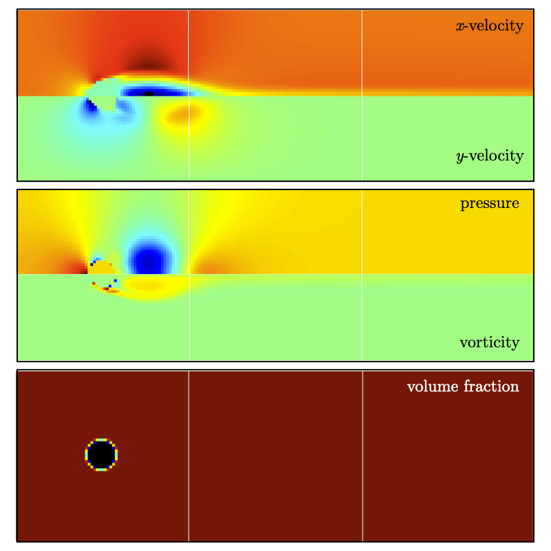 |
At this point, you have established a flow with a large recirculation zone in the wake of the cylinder, but the flow has not yet fully transitioned to periodic vortex shedding. The flow is depicted in Fig 5 showing a few of the available contour plots at 50 ms. Note that the value of the fully covered cells is set to zero.
As can be seen from Fig 5, the flow has not yet transitioned to the familiar Von-Karman alleys and two aspects of the current simulation can delay or even prevent the onset of vortex shedding:
- the flow is initially symmetric and the transition to the familiar periodic flow is due to the growth of infinitesimal perturbations in the shear layer of the wake. Because the flow is artificially too symmetric, this transition can be delayed until round-off errors sufficiently accumulate.
- the numerical dissipation introduced by this coarse grid results in an effective Reynolds number probably significantly lower than the value estimated above.
Before adding refinement levels, we will first pursue the simulation until the flow reaches a periodic vortex shedding state. To do so, restart the simulation from the checkpoint file generated at the end of the first run and set the final simulation time to 200 ms:
#-------------------------IO CONTROL----------------------------
...
amr.restart             = chk_01327 # Restart from checkpoint ?

...

#----------------------TIME STEPING CONTROL----------------------
...
stop_time      = 0.20            # final physical time
and restart the simulation
./PeleLM2d.gnu.MPI.ex inputs.2d-regt_VS > logCoarseRun2.dat &
The flow has now fully transition and you can use Amrvis to visualize the serie of vortex in the wake of the cylinder. In the next step, we will add finer grid patches around the EB geometry and in high vorticity regions.
Refinement of the computation
We will now add a first level of refinement. In the present simulation, the refinement criteria could be based on several characteristics of the flow: velocity gradients, vorticity, pressure, … In the following, we will simply use vorticity.
Additionally, by construction the geometry must be built to the finest level which act as a refinement criteria based on the gradient of volume fraction. This is beneficial in this case in order to help refine the cylinder boundary layer.
Start by increasing the number of AMR levels to one in the AMR CONTROL block:
amr.max_level = 1 # maximum level number allowed
Then provide a definition of the new refinement critera in the REFINEMENT CONTROL block:
#--------------------REFINEMENT CONTROL------------------------
# Refinement according to the vorticity, no field_name needed
amr.refinement_indicators     = lowvort highvort
amr.lowvort.max_level         = 1
amr.lowvort.value_less        = -1000
amr.lowvort.field_name        = mag_vort

amr.highvort.max_level         = 1
amr.highvort.value_greater     = 1000
amr.highvort.field_name        = mag_vort

# Refine the EB
ns.refine_cutcells            = 1
The first line simply declares a set of refinement indicators which are subsequently defined. For each indicator, the user can provide a limit up to which AMR level this indicator will be used to refine. Then there are multiple possibilities to specify the actual criterion: value_greater, value_less, vorticity_greater or adjacent_difference_greater. In each case, the user specify a threshold value and the name of variable on which it applies (except for the vorticity_greater).
In the example above, the grid is refined up to level 1 at the location where the vorticity magnitude is above 1000 \(s^{-1}\) as well as on the cut cells (where the cylinder intersect with the edges of cell). Note that in the present case, the vorticity_greater was not used to ensure that regions of both low and high vorticity are refined.
With these new parameters, change the checkpoint file from which to restart and allow regridding upon restart by updating the following lines in the IO CONTROL block:
amr.restart             = chk_06195 # Restart from checkpoint ?
amr.regrid_on_restart   = 1
, increase the stop_time to 300 ms in the TIME STEPING CONTROL block:
stop_time = 0.30 # final physical time
and start the simulation again (using multiple processor if available)
mpirun -n 4 ./PeleLM2d.gnu.MPI.ex inputs.2d-regt_VS > log2Levels.dat &
Once again, use Amrvis to visualize the effects of refinement: after an initial transient, the flow return to a smooth periodic vortex shedding and the boundary layer of the cylinder is now significantly better captured but still far from fully refined. As a final step, we will add another level of refinement, only at the vicinity of the cylinder since the level 1 resolution appears sufficient to discretize the vortices in the wake. To do so, simply allow for another level of refinement:
amr.max_level = 2 # maximum level number allowed
and since the vorticity refinement criterion only refine up to level 1, the level 2 will only be located around the EB. Update the checkpoint file in the IO CONTROL block, increase the stop_time to 350 ms in the the TIME STEPING CONTROL and restart the simulation:
mpirun -n 4 ./PeleLM2d.gnu.MPI.ex inputs.2d-regt_VS > log3Levels.dat &
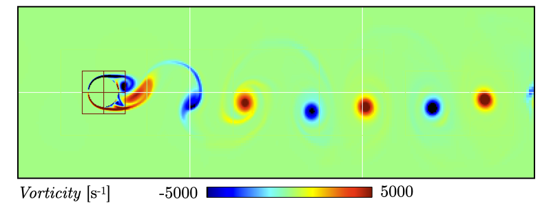
You should obtain a flow with a vorticity field similar to Fig. 6. For the purpose of the present tutorial, this will be our final solution but one can see that the flow has not yet return to a periodic vortex shedding and additinal resolution could be added locally to obtain smoother flow features.
 |