Tutorial - A simple triple flame
Introduction
Laminar flames have the potential to reveal the fundamental structure of combustion without the added complexities of turbulence. They also aid in our understanding of the more complex turbulent flames. Depending on the fuel involved and the flow configuration, the laminar flames can take on a number of interesting geometries. For example, as practical combustion systems often operate in partially premixed mode, with one or more fuel injections, a wide range of fresh gas compositions can be observed; and these conditions favor the appearance of edge flames, see Fig. 7.
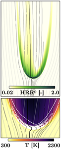 |
Edge flames are composed of lean and rich premixed flame wings usually surrounding a central anchoring diffusion flame extending from a single point [PCI2007]. Edge flames play an important role in flame stabilization, re-ignition and propagation. Simple fuels can exhibit up to three burning branches while diesel fuel, with a low temperature combustion mode, can exhibit up to 5 branches.
The goal of this tutorial is to setup a simple 2D laminar triple edge flame configuration with PeleLM. This document provides step by step instructions to properly set-up the domain and boundary conditions, construct an initial solution, and provides guidance on how to monitor and influence the initial transient to reach a final steady-state solution. In a final Section, post-processing tools available in PeleAnalysis are used to extract information about the triple flame.
Setting-up your environment
PeleProduction
As explained in section PeleLM Quickstart, PeleLM relies on a number of supporting softwares:
- AMReX is a software frameworks that provides the data structure and enable massive parallelization.
- AMReX-Hydro is a suite of AMReX-based fonctionalities handling the hydrodynamic schemes.
- IAMR is a parallel, adaptive mesh refinement (AMR) code that solves the variable-density incompressible Navier-Stokes equations.
- PelePhysics is a repository of physics databases and implementation code. In particular, the choice of chemistry and transport models as well as associated functions and capabilities are managed in PelePhysics.
All of these codes have their own development cycle, and it can make the setup of a PeleLM run a bit tricky. To simplify the process, PeleProduction will be employed. PeleProduction is a collection of run folders for various Pele codes and processing. It includes git submodules for the dependent codes (such as PeleLM, PelePhysics, AMReX, etc), that can be frozen to a particular commit. This organizational strategy enables to manage the interactions between the various dependent repositories (to keep them all compatible with each other).
Step by step instructions
First, make sure that “git” is installed on your machine—we recommend version 1.7.x or higher. Then, follow these few steps to setup your run environment:
Download the PeleProduction repository and :
git clone https://github.com/AMReX-Combustion/PeleProduction.git

cd PeleProduction
Switch to the TripleFlame branch :
git checkout -b Tutorials remotes/origin/Tutorials
The first time you do this, you will need to tell git that there are submodules. Git will look at the
.gitmodulesfile in this branch and use that :git submodule init
Finally, get the correct commits of the sub-repos set up for this branch:
git submodule update
You are now ready to build the TripleFlame case associated with this branch. To do so:
cd Tutorials/TripleFlame
And follow the next steps !
Numerical setup
In this section we review the content of the various input files for the Triple Flame test case. To get additional information about the keywords discussed, the user is referred to section PeleLM control.
Test case and boundary conditions
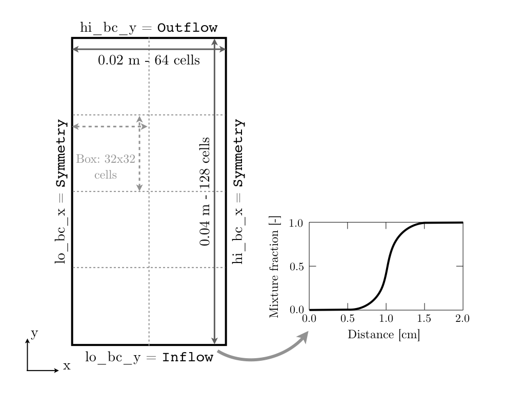
Direct Numerical Simulations (DNS) are performed on a 2x4 \(cm^2\) 2D computational domain using a 64x128 base grid and up to 4 levels of refinement (although we will start with a lower number of levels). The refinement ratio between each level is set to 2. With 4 levels, this means that the minimum grid size inside the reaction layer will be just below 20 \(μm\). The maximum box size is fixed at 32, and the base (level 0) grid is composed of 8 boxes, as shown in Fig 8.
Symmetric boundary conditions are used in the transverse (\(x\)) direction, while Inflow (dirichlet) and Outflow (neumann) boundary conditions are used in the main flow direction (\(y\)). The flow goes from the bottom to the top of the domain. The specificities of the Inflow boundary condition are explained in subsection Inflow specification
 |
The geometry of the problem is specified in the first block of the inputs.2d-regt:
#----------------------DOMAIN DEFINITION------------------------
geometry.is_periodic = 0 0       # Periodicity in each direction: 0 => no, 1 => yes
geometry.coord_sys   = 0         # 0 => cart, 1 => RZ
geometry.prob_lo     = 0. 0.     # x_lo y_lo
geometry.prob_hi     = 0.02 0.04 # x_hi y_hi
The second block determines the boundary conditions. Refer to Fig 8:
# >>>>>>>>>>>>>  BC FLAGS <<<<<<<<<<<<<<<<
# Interior, Inflow, Outflow, Symmetry,
# SlipWallAdiab, NoSlipWallAdiab, SlipWallIsotherm, NoSlipWallIsotherm
peleLM.lo_bc = Symmetry  Inflow
peleLM.hi_bc = Symmetry  Outflow
The number of levels, refinement ratio between levels, maximium grid size as well as other related refinement parameters are set under the third block :
#-------------------------AMR CONTROL----------------------------
amr.n_cell          = 64 128     # Level 0 number of cells in each direction
amr.v               = 1          # amr verbosity level
amr.max_level       = 1          # maximum level number allowed
amr.ref_ratio       = 2 2 2 2    # refinement ratio
amr.regrid_int      = 2          # how often to regrid
amr.n_error_buf     = 1 1 1 2    # number of buffer cells in error est
amr.grid_eff        = 0.9        # what constitutes an efficient grid
amr.grid_eff        = 0.7        # what constitutes an efficient grid
amr.blocking_factor = 16         # block factor in grid generation
amr.max_grid_size   = 32         # maximum box size
Inflow specification
The edge flame is stabilized against an incoming mixing layer with a uniform velocity profile. The mixing layer is prescribed using an hyperbolic tangent of mixture fraction \(z\) between 0 and 1, as can be seen in Fig 8:
where \(z\) is based on the classical elemental composition [CF1990]:
where \(\beta\) is Bilger’s coupling function, and subscript \(ox\) and \(fu\) correspond to oxidizer and fuel streams respectively.
Specifying dirichlet Inflow conditions in PeleLM can seem daunting at first. But it is actually a very flexible process. We walk the user through the details of it for the Triple Flame case just described. The files involved are:
pelelm_prob_parm.H, assemble in a C++ namespaceProbParmthe input variables as well as other variables used in the initialization process.pelelm_prob.cpp, initialize and provide default values to the entries ofProbParmand allow the user to pass run-time value using the AMReX parser (ParmParse). In the present case, the parser will read the parameters in thePROBLEM PARAMETERSblock:prob.P_mean = 101325.0 prob.T_in = 300.0 prob.V_in = 0.85 prob.Zst = 0.055
finally,
pelelm_prob.Hcontains thepelelm_initdataandbcnormalfunctions responsible for generating the initial and boundary conditions, resspectively.
Note that in our specific case, we compute the input value of the mass fractions (Y) directly in bcnormal, using the ProbParm variables. We do not need any additional information, because we hard coded the hyperbolic tangent profile of \(z\) (see previous formula) and there is a direct relation with the mass fraction profiles. The interested reader can look at the function set_Y_from_Ksi and set_Y_from_Phi in pelelm_prob.H.
Initial solution
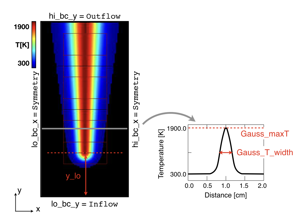
An initial field of the main variables is always required to start a simulation. Ideally, you want for this initial solution to approximate the final (steady-state in our case) solution as much as possible. This will speed up the initial transient and avoid many convergence issues. In the present tutorial, an initial solution is constructed by imposing the same inlet hyperbolic tangent of mixture fraction than described in subsection Inflow specification everywhere in the domain; and reconstructing the species mass fraction profiles from it. To ensure ignition of the mixture, a progressively widening Gaussian profile of temperature is added, starting from about 1 cm, and stretching until the outlet of the domain. The initial temperature field is shown in Fig 9, along with the parameters controlling the shape of the hot spot.
 |
This initial solution is constructed via the routine pelelm_initdata(), in the file pelelm_prob.H. Additional information is provided as comments in this file for the eager reader, but nothing is required from the user at this point.
Numerical scheme
The NUMERICS CONTROL block can be modified by the user to increase the number of SDC iterations. Note that there are many other parameters controlling the numerical algorithm that the advanced user can tweak, but we will not talk about them in the present Tutorial. The interested user can refer to section PeleLM algorithm controls.
Building the executable
The last necessary step before starting the simulation consists of building the PeleLM executable. AMReX applications use a makefile system to ensure that all the required source code from the dependent libraries be properly compiled and linked. The GNUmakefile provides some compile-time options regarding the simulation we want to perform. The first four lines of the file specify the paths towards the source code of PeleLM, AMReX, IAMR and PelePhysics and should not be changed.
Next comes the build configuration block:
#
# Build configuration
#
DIM             = 2
COMP            = gnu
DEBUG           = FALSE
USE_MPI         = TRUE
USE_OMP         = FALSE
USE_CUDA        = FALSE
PRECISION       = DOUBLE
VERBOSE         = FALSE
TINY_PROFILE    = FALSE
It allows the user to specify the number of spatial dimensions (2D), the compiler (gnu) and the parallelism paradigm (in the present case only MPI is used). The other options can be activated for debugging and profiling purposes.
In PeleLM, the chemistry model (set of species, their thermodynamic and transport properties as well as the description of their of chemical interactions) is specified at compile time. Chemistry models available in PelePhysics can used in PeleLM by specifying the name of the folder in PelePhysics/Support/Fuego/Mechanisms/Models containing the relevant files, for example:
Chemistry_Model = drm19
Here, the methane kinetic model drm19, containing 21 species is employed. The user is referred to the PelePhysics documentation for a list of available mechanisms and more information regarding the EOS, chemistry and transport models specified:
Eos_Model       := Fuego
Transport_Model := Simple
Finally, PeleLM utilizes the chemical kinetic ODE integrator CVODE. This Third Party Librabry (TPL) is not shipped with the PeleLM distribution but can be readily installed through the makefile system of PeleLM. To do so, type in the following command:
make TPL
Note that the installation of CVODE requires CMake 3.12.1 or higher.
You are now ready to build your first PeleLM executable !! Type in:
make -j4
The option here tells make to use up to 4 processors to create the executable (internally, make follows a dependency graph to ensure any required ordering in the build is satisfied). This step should generate the following file (providing that the build configuration you used matches the one above):
PeleLM2d.gnu.MPI.ex
You’re good to go !
Initial transient phase
First step: the initial solution
When performing time-dependent numerical simulations, it is good practice to verify the initial solution. To do so, we will run PeleLM for a single time step, to generate an initial plotfile plt_00000.
Time-stepping parameters in input.2d-regt are specified in the TIME STEPING CONTROL block:
#----------------------TIME STEPING CONTROL----------------------
max_step       = 1               # maximum number of time steps
stop_time      = 4.00            # final physical time
ns.cfl         = 0.1             # cfl number for hyperbolic system
ns.init_shrink = 0.01            # scale back initial timestep
ns.change_max  = 1.1             # max timestep size increase
ns.dt_cutoff   = 5.e-10          # level 0 timestep below which we halt
The maximum number of time steps is set to 1 for now, while the final simulation time is 4.0 s. Note that, when both max_step and stop_time are specified, the more stringent constraint will control the termination of the simulation. PeleLM solves for the advection, diffusion and reaction processes in time, but only the advection term is treated explicitly and thus it constrains the maximum time step size \(dt_{CFL}\). This constraint is formulated with a classical Courant-Friedrich-Levy (CFL) number, specified via the keyword ns.cfl. Additionally, as it is the case here, the initial solution is often made-up by the user and local mixture composition and temperature can result in the introduction of unreasonably fast chemical scales. To ease the numerical integration of this initial transient, the parameter ns.init_shrink allows to shrink the inital dt (evaluated from the CFL constraint) by a factor (usually smaller than 1), and let it relax towards \(dt_{CFL}\) as the simulation proceeds.
Input/output from PeleLM are specified in the IO CONTROL block:
#-------------------------IO CONTROL----------------------------
#amr.restart           = chk01000 # Restart from checkpoint ?
#amr.regrid_on_restart = 1        # Perform regriding upon restart ?
amr.checkpoint_files_output = 0   # Dump check file ? 0: no, 1: yes
amr.check_file      = chk         # root name of checkpoint file
amr.check_int       = 100         # number of timesteps between checkpoints
amr.plot_file       = plt         # root name of plotfiles
amr.plot_int        = 20          # number of timesteps between plotfiles
amr.derive_plot_vars=rhoRT mag_vort avg_pressure gradpx gradpy diveru mass_fractions mixfrac
amr.grid_log        = grdlog      # name of grid logging file
The first two lines (commented out for now) are only used when restarting a simulation from a checkpoint file and will be useful later during this tutorial. Information pertaining to the checkpoint and plot_file files name and output frequency can be specified there. PeleLM will always generate an initial plotfile plt_00000 if the initialization is properly completed, and a final plotfile at the end of the simulation. It is possible to request including derived variables in the plotfiles by appending their names to the amr.derive_plot_vars keyword. These variables are derived from the state variables (velocity, density, temperature, \(\rho Y_k\), \(\rho h\)) which are automatically included in the plotfile. Note also that the name of the probin file used to specify the initial/boundary conditions is defined here.
You finally have all the information necessary to run the first of several steps to generate a steady triple flame. Type in:
./PeleLM2d.gnu.MPI.ex inputs.2d-regt
A lot of information is printed directly on the screen during a PeleLM simulation, but it will not be detailed in the present tutorial. If you wish to store these information for later analysis, you can instead use:
./PeleLM2d.gnu.MPI.ex inputs.2d-regt > logCheckInitialSolution.dat &
Whether you have used one or the other command, within 30 s you should obtain a plt_00000 and a plt_00001 files (or even more, appended with .old*********** if you used both commands). Use Amrvis to vizualize plt_00000 and make sure the solution matches the one shown in Fig. 9.
Running the problem on a coarse grid
As mentioned above, the initial solution is relatively far from the steady-state triple flame we wish to obtain. An inexpensive and rapid way to transition from the initial solution to an established triple flame is to perform a coarse (using only 2 AMR levels) simulation using a single SDC iteration for a few initial number of time steps (here we start with 1000). To do so, update (or verify !) these associated keywords in the input.2d-regt:
#-------------------------AMR CONTROL----------------------------
...
amr.max_level     = 1             # maximum level number allowed
...
#----------------------TIME STEPING CONTROL----------------------
...
max_step          = 1000          # maximum number of time steps
...
#--------------------NUMERICS CONTROL------------------------
...
ns.sdc_iterMAX    = 1             # Number of SDC iterations
In order to later on continue the simulation with refined parameters, we need to trigger the generation of a checkpoint file, in the IO CONTROL block:
amr.checkpoint_files_output = 1 # Dump check file ? 0: no, 1: yes
To be able to complete this first step relatively quickly, it is advised to run PeleLM using at least 4 MPI processes. It will then take a couple of hours to reach completion. To be able to monitor the simulation while it is running, use the following command:
mpirun -n 4 ./PeleLM2d.gnu.MPI.ex inputs.2d-regt > logCheckInitialTransient.dat &
A plotfile is generated every 20 time steps (as specified via the amr.plot_int keyword in the IO CONTROL block). This will allow you to visualize and monitor the evolution of the flame. Use the following command to open multiple plotfiles at once with Amrvis:
amrvis -a plt????0
An animation of the flame evolution during this initial transient is provided in Fig 10.
Steady-state problem: activating the flame control
The speed of propagation of a triple flame is not easy to determine a-priori. As such it is useful, at least until the flame settles, to have some sort of stabilization mechanism to prevent flame blow-off or flashback. In the present configuration, the position of the flame front can be tracked at each time step (using an isoline of temperature) and the input velocity is adjusted to maintain its location at a fixed distance from the inlet (1 cm in the present case).
The parameters of the active control are listed in INPUTS TO ACTIVE CONTROL block of inputs.2d-regt:
# --------------  INPUTS TO ACTIVE CONTROL  -----------------
active_control.on = 1                  # Use AC ?
active_control.use_temp = 1            # Default in fuel mass, rather use iso-T position ?
active_control.temperature = 1400.0    # Value of iso-T ?
active_control.tau = 1.0e-4            # Control tau (should ~ 10 dt)
active_control.height = 0.01           # Where is the flame held ? Default assumes coordinate along Y in 2D or Z in 3D.
active_control.v = 1                   # verbose
active_control.velMax = 2.0            # Optional: limit inlet velocity
active_control.changeMax = 0.1         # Optional: limit inlet velocity changes (absolute)
active_control.flameDir  = 1           # Optional: flame main direction. Default: AMREX_SPACEDIM-1
active_control.pseudo_gravity = 1      # Optional: add density proportional force to compensate for the acceleration
                                       #           of the gas due to inlet velocity changes
The first keyword activates the active control and the second one specify that the flame will be tracked based on an iso-line of temperature, the value of which is provided in the third keyword. The following parameters controls the relaxation of the inlet velocity to
the steady state velocity of the triple flame. tau is a relaxation time scale, that should be of the order of ten times the simulation time-step.
height is the user-defined location where the triple flame should settle, changeMax and velMax control the maximum velocity increment and maximum inlet velocity, respectively. The user is referred to [CAMCS2006] for an overview of the method and corresponding parameters.
The pseudo_gravity triggers a manufactured force added to the momemtum equation to compensate for the acceleration of different density gases.
Once these paremeters are set, you continue the previous simulation by uncommenting the first two lines of the IO CONTROL block in the input file:
amr.restart           = chk01000 # Restart from checkpoint ?
amr.regrid_on_restart = 1        # Perform regriding upon restart ?
The first line provides the last checkpoint file generated during the first simulation performed for 1000 time steps. Note that the second line, forcing regriding of the simulation upon restart, is not essential at this point. Finally, update the max_step to allow the simulation to proceed further:
#----------------------TIME STEPING CONTROL----------------------
...
max_step          = 2000          # maximum number of time steps
You are now ready launch PeleLM again for another 1000 time steps !
mpirun -n 4 ./PeleLM2d.gnu.MPI.ex inputs.2d-regt > logCheckControl.dat &
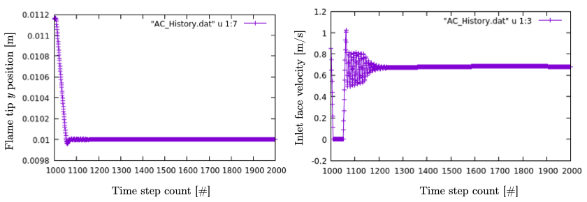
As the simulation proceeds, an ASCII file tracking the flame position and inlet velocity (as well as other control variables) is generated: AC_History. You can follow the motion of the flame tip by plotting the eigth column against the first one (flame tip vs. time step count). If gnuplot is available on your computer, use the following to obtain the graphs of Fig 11:
gnuplot
plot "AC_History.dat" u 1:7 w lp
plot "AC_History.dat" u 1:3 w lp
exit
The second plot corresponds to the inlet velocity.
 |
At this point, you have a stabilized methane/air triple flame and will now use AMR features to improve the quality of your simulation.
Refinement of the computation
Before going further, it is important to look at the results of the current simulation. The left panel of Fig. 12 displays the temperature field, while a zoom-in of the flame edge region colored by several important variables is provided on the right side. Note that DivU, the HeatRelease and the CH4_consumption are good markers of the reaction/diffusion processes in our case. What is striking from these images is the lack of resolution of the triple flame, particularly in the reaction zone. We also clearly see square unsmooth shapes in the field of intermediate species, where Y(HCO) is found to closely match the region of high CH4_consumption while Y(CH3O) is located closer to the cold gases, on the outer layer of the triple flame.
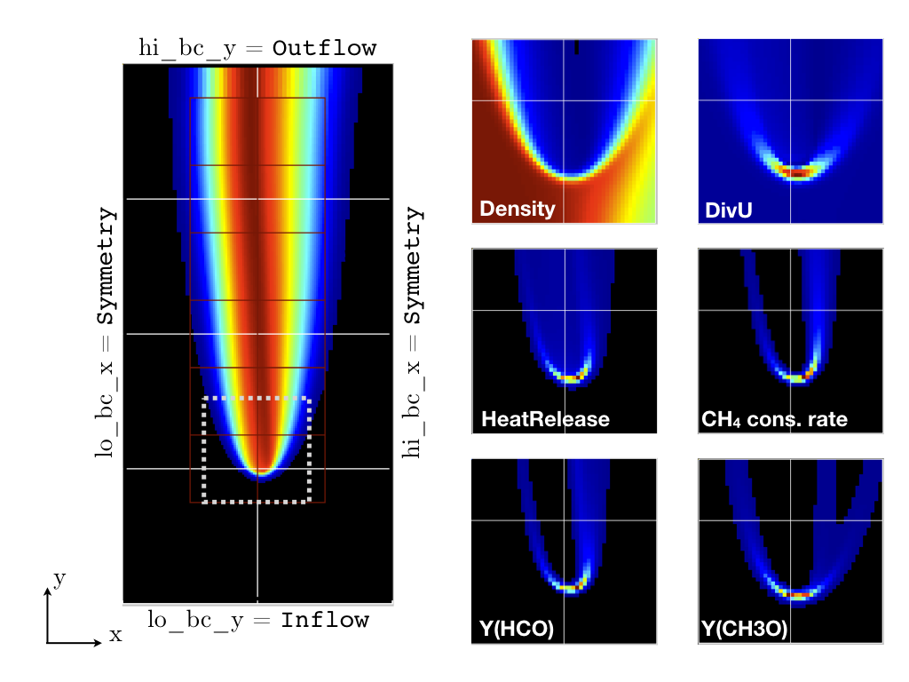 |
Our first level of refinement must specifically target the reactive layer of the flame. As seen from Fig. 12, one can choose from several variables to reach that goal. In the following, we will use the CH3O species as a tracer of the flame position. Start by increasing the number of AMR levels by one in the AMR CONTROL block:
amr.max_level = 2 # maximum level number allowed
Then provide a definition of the new refinement critera in the REFINEMENT CONTROL block:
#--------------------REFINEMENT CONTROL------------------------
amr.refinement_indicators = hi_temp gradT flame_tracer   # Declare set of refinement indicators

amr.hi_temp.max_level     = 1
amr.hi_temp.value_greater = 800
amr.hi_temp.field_name    = temp

amr.gradT.max_level                   = 1
amr.gradT.adjacent_difference_greater = 200
amr.gradT.field_name                  = temp

amr.flame_tracer.max_level     = 2
amr.flame_tracer.value_greater = 1.0e-6
amr.flame_tracer.field_name    = Y(CH3O)
The first line simply declares a set of refinement indicators which are subsequently defined. For each indicator, the user can provide a limit up to which AMR level this indicator will be used to refine. Then there are multiple possibilities to specify the actual criterion: value_greater, value_less, vorticity_greater or adjacent_difference_greater. In each case, the user specify a threshold value and the name of variable on which it applies (except for the vorticity_greater). In the example above, the grid is refined up to level 1 at the location wheres the temperature is above 800 K or where the temperature difference between adjacent cells exceed 200 K. These two criteria were used up to that point. The last indicator will now enable to add level 2 grid patches at location where the flame tracer (Y(CH3O)) is above 1.0e-6.
With these new parameters, update the checkpoint file from which to restart:
amr.restart = chk02000 # Restart from checkpoint ?
and increase the max_step to 2300 and start the simulation again !
mpirun -n 4 ./PeleLM2d.gnu.MPI.ex inputs.2d-regt > log3Levels.dat &
Visualization of the 3-levels simulation results indicates that the flame front is now better repesented on the fine grid, but there are still only a couple of cells across the flame front thickness. The flame tip velocity, captured in the AC_history, also exhibits a significant change with the addition of the third level (even past the initial transient). In the present case, the flame tip velocity is our main quantity of interest and we will now add another refinement level to ensure that this quantity is fairly well capture. We will use the same refinement indicators and simply update the max_level as well as the level at which each refinement criteria is used:
amr.max_level       = 3          # maximum level number allowed

...

amr.restart           = chk02300 # Restart from checkpoint ?

...

amr.gradT.max_level                   = 2

...

amr.flame_tracer.max_level     = 3
and increase the max_step to 2600. The temporal evolution of the inlet velocity also shows that our active control parameters induce rather strong oscillations of the velocity before it settles. To illustrate how we can tune the AC parameters to limit this behavior, we will increase the tau parameter:
active_control.tau = 4.0e-4 # Control tau (should ~ 10 dt)
Let’s start the simulation again !
mpirun -n 4 ./PeleLM2d.gnu.MPI.ex inputs.2d-regt > log4Levels.dat &
Finally, we will now improve PeleLM algorithm accuracy itself. So far, for computational expense reasons, we have only used a single SDC iteration which provide a relatively weak coupling between the slow advection and the fast diffusion/reaction processes, as well as a loose enforcement of the velocity divergence constrain (see PeleLM description for more information). We will now increase the number of SDC iteration to two, allowing to reach the theoretical second order convergence property of the algorithm:
#--------------------NUMERICS CONTROL------------------------
 ...
 ns.sdc_iterMAX    = 2             # Number of SDC iterations
and further continue the simulation to reach 2800 time steps. Note that, as with an increase of the maximum refinement level, increasing the number of SDC iterations incurs a significant increase of the computational time per coarse time step. Let’s complete this final step:
mpirun -n 4 ./PeleLM2d.gnu.MPI.ex inputs.2d-regt > log4Levels_2SDC.dat &
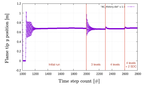
Figure 13 shows the entire history of the inlet velocity starting when the AC was activated (1000th time step). We can see that every change in the numerical setup induced a slight change in the triple flame propagation velocity, eventually leading to a nearly constant value, sufficient for the purpose of this tutorial.
 |
At this point, the simulation is considered complete and the next section provide some pointer to further analyze the results.
Analysis
| [PCI2007] |
|
| [CF1990] |
|
| [CAMCS2006] |
|